EXTRACT FROM INTRODUCITON: We model lakes to visualize and quantify fluid flow, mass transport, and thermal structure. Understanding the evolving physical state (e.g., surface elevation, density, temperature, velocity, turbidity) is necessary for modeling fluxes of nutrients, pollutants, or biota in time-varying fields of one, two, or three space dimensions (1D, 2D, or 3D). Hydrodynamic modeling provides insight into spatial–temporal changes in physical processes seen in field data. For example, Figure 1 shows temperature profiles simultaneously recorded at different stations around Lake Kinneret (Israel). Extracts from model results (Figure 2) provides a context for interpreting these data as a coherent tilting of the thermocline. A time series of the thermocline can be animated, showing the principal motion is a counter-clockwise rotation of the thermocline. The complexities of the thermocline motion can be further dissected by using spectral signal processing techniques to separate wave components, illustrating a basin-scale Kelvin wave, a first-mode Poincare´ wave, and a second-mode Poincare´ wave.

EXTRACT: Figure 1.

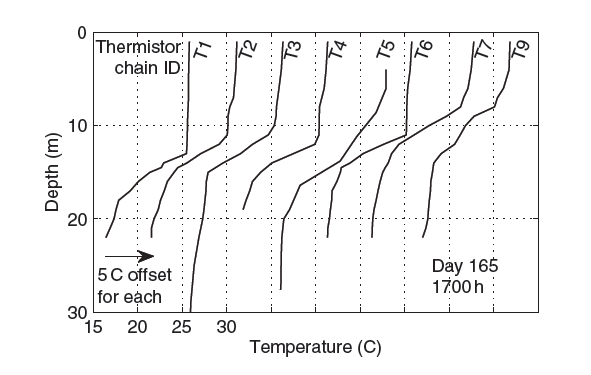
Figure 1. Temperature profiles collected in Lake Kinneret in 1997 (data of J. Imberger, Centre for Water Research, University of Western Australia).

EXTRACT: Figure 2.

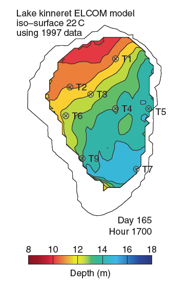
Figure 2. Modeled depth of temperature isosurface in the thermocline. Results from 3D-model at same time as field data collected in Figure 1.